Understanding the scan operation

\[\newcommand{\bigO}{\mathcal{O}}\]

When we develop algorithms and numerical methods, we often find ourselves with the same concern when it comes to scalability. If we want a method to be practical and have impact on large scale (real-world) problems, we need to ensure it runs fast. Parallelizing algorithms is a way to greatly accelerate their execution speed. The fact is that some algorithms are easily and obviously parallelizable, while others simply cannot be.

In this post, we focus on a specific type of operation – that can be part of many algorithms – and explore how it can be parallelized through a technique called the scan operation.

What is the scan operation?

The scan operation takes a sequence as input and produces a new sequence as output. In this blog, we choose to use the word “sequence” instead of “array” or “list” to emphasize on the structure of the output, which is a sequence of values that are derived from the input sequence. Let’s say that we are given a sequence of elements $x$ of length $n$:

\[x = [x_0, x_1, \ldots, x_{n-1}],\]

and an associative¹ operator $\oplus$; then the scan operation is interested in computing the following output sequence:

\[y = [y_0, y_1, \ldots, y_{n-1}],\]

where each element is defined as:

\[y_i = x_0 \oplus x_1 \oplus \ldots \oplus x_i, \quad 0 \leq i < n.\]

This means that the $i$-th element of the output sequence $y$ is the result of applying the operator $\oplus$ to all elements of the input sequence $x$ from index $0$ to index $i$:

\[x = [x_0, x_1, \ldots, x_{n-1}] \overset{\mathrm{scan}(\oplus)}{\longrightarrow} y = [x_0, x_0 \oplus x_1, x_0 \oplus x_1 \oplus x_2, \ldots, x_0 \oplus x_1 \oplus \ldots \oplus x_{n-1}].\]

The scan operation² is particularly useful when we want to parallelize computations of the output sequence $y$ from the input sequence $x$³.

How to parallelize the scan operation?

The hot question of the day is: how can we parallelize the scan operation? Indeed, when we look at the definition of the output sequence $y$, we see that each element $y_i$ depends on all previous elements $x_0, x_1, \ldots, x_i$. This means that if we were to compute the scan operation in a very very naive way, we would have to compute each element sequentially, which would take $\bigO(n^2)$ time in the worst case. Let’s understand this with a C code example:

# | title: Naive O(n^2) scan implementation
void naive_scan_On2(double *input, double *output, int n, double (*op)(double, double)) {
    for (int i = 0; i < n; i++) {
        output[i] = input[0];
        for (int j = 1; j <= i; j++) {
            output[i] = op(output[i], input[j]);
        }
    }
}

The operator that we are considering in this blog post is constructed to be quite computationally expensive, so that we are able to see the difference between the different implementations and we are less impacted by the overhead of the function calls and the memory accesses. The operator is defined as follows:

# | title: Expensive operator
#define ITER 250
double op(double a, double b) { 
    for (int i = 0; i < ITER; ++i) {
        a = a*a - 0.5*a + 0.1;
        b = b*b - 0.5*b + 0.1;
    }
    return a + b;
}

One can check that this is indeed an associative operator. If we run the naive implementation on different input sizes, we can observe the following time complexity:

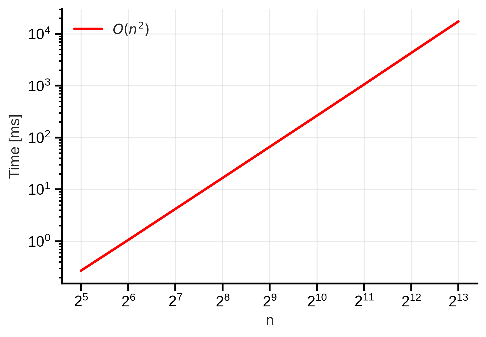Figure 1: Naive O(n²) scan time complexity. We observe that the time taken increases quadratically with the input size. The shaded area shows the min-max variability across 5 different runs. One should note that we always use a log-log scale for both axes.

Of course, this is not a practical implementation for large inputs, as it has a time complexity of $\bigO(n^2)$. One can do better even without any parallelization, by simply observing that each element $y_i$ can be computed as: $y_i = y_{i-1} \oplus x_i$, which leads to a linear time complexity $\bigO(n)$:

# | title: (Still naive) O(n) scan implementation
void naive_scan_On(double *input, double *output, int n, double (*op)(double, double)) {
    output[0] = input[0];
    for (int i = 1; i < n; i++) {
        output[i] = op(output[i - 1], input[i]);
    }
}

Empirically, we observe that this implementation has a linear time complexity: 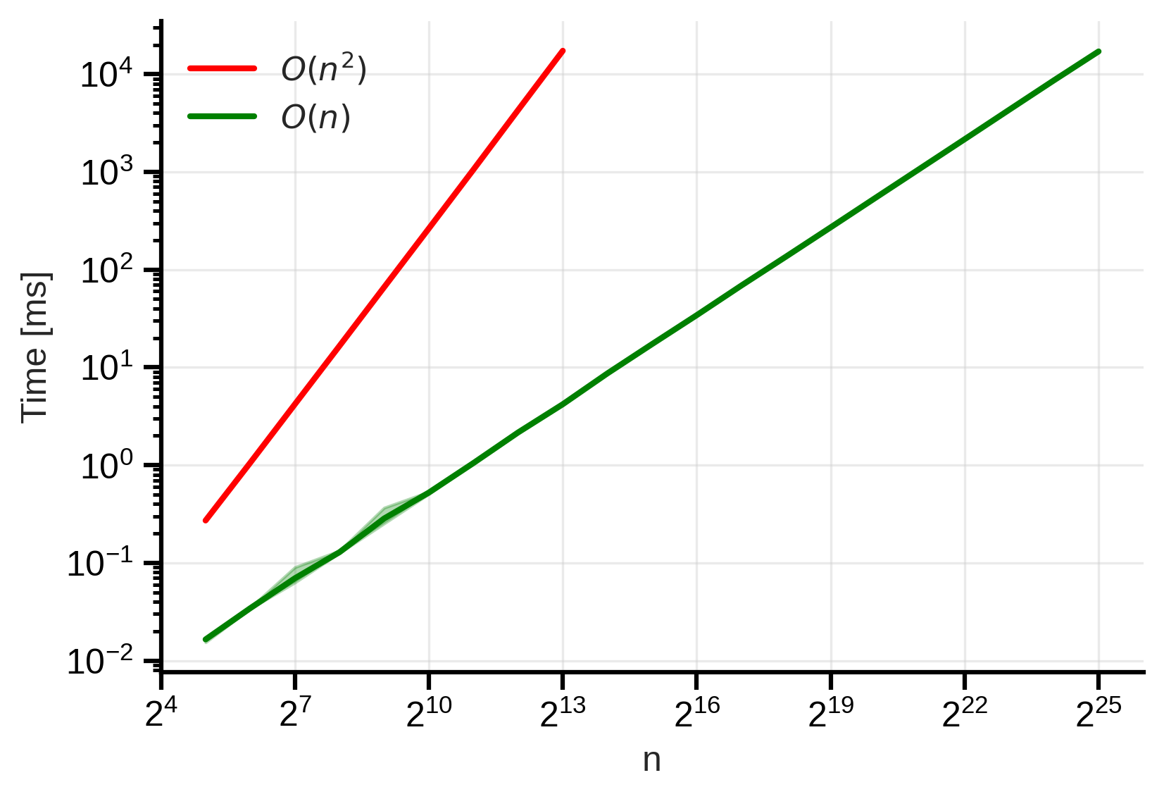Figure 2: Naive O(n) scan time complexity. We observe that the time taken increases linearly with the input size. The shaded area shows the min-max variability across 5 different runs.

Here we have reduced the time complexity by reducing the work complexity. Before diving into parallelization, let’s first understand the difference between these two concepts.

Work complexity vs time complexity

The time complexity of an algorithm is the total amount of time it takes to execute the algorithm and get the result. We express complexity using the big-O notation, which gives us an idea of the type of growth of the time taken by the algorithm as the input size increases. Let’s say that we have a first algorithm with a time complexity of $\bigO(n^2)$ and a second algorithm with a time complexity of $\bigO(n)$. Given two input sequences of size $n$ and $2n$, the first algorithm will take about $4$ times more time when processing the second input sequence compared to the first sequence, while the second algorithm will take about $2$ times more time.

Intuitively, one thing that makes some algorithms faster than others is the amount of operations they perform. This is what we call the work complexity of an algorithm. The work complexity is the total number of operations performed by the algorithm, regardless of how long each operation takes. For example, the naive scan implementation has a work complexity of $\bigO(n^2)$, while the “improved” version has a work complexity of $\bigO(n)$.

— So there is no difference between work complexity and time complexity? If I perform the same number of operations, for sure the time that I will take will be the same, right?

Not quite. The time complexity is the total time taken by the algorithm, while the work complexity is the total number of operations performed by the algorithm. The time complexity depends on the work complexity, but also on the parallelism of the algorithm. If an algorithm can perform multiple operations in parallel (i.e., at the same time), then the time complexity can be reduced even further.

The central question in parallel computing is: given more processing units, can I reduce the time complexity of my algorithm? The answer is yes, but it depends on the algorithm and the type of operations it performs.

The scan operation is not purely sequential

Even if the scan operation is defined in a sequential way, it is not purely sequential. Indeed, we do have the full input sequence $x$ available at the beginning of the computation, and we can compute the output sequence $y$ in a way that does not require us to wait for the previous elements to be computed. There are two main ways to parallelize the scan operation: the Hillis-Steele algorithm and the Blelloch algorithm. Both algorithms are based on the idea of divide and conquer, but they differ in how they handle the input sequence and the output sequence.

We start with the Hillis-Steele algorithm that is easier to understand but that is not as work-efficient as the Blelloch algorithm – however, both algorithms have the same time complexity.

The Hillis-Steele algorithm

The Hillis-Steele algorithm can be understood through a tree structure. This tree is purely conceptual, that is, we are not going to implement it as a tree data structure, but rather as a sequence of operations that can be performed in parallel. The tree will have a depth of $\lceil\log_2(n)\rceil$. At each level $d$ of the tree, we will apply the $\oplus$ operator on $n-2^d$ elements in parallel and don’t touch to the remaining $2^d$ elements. The tree structure is as follows:

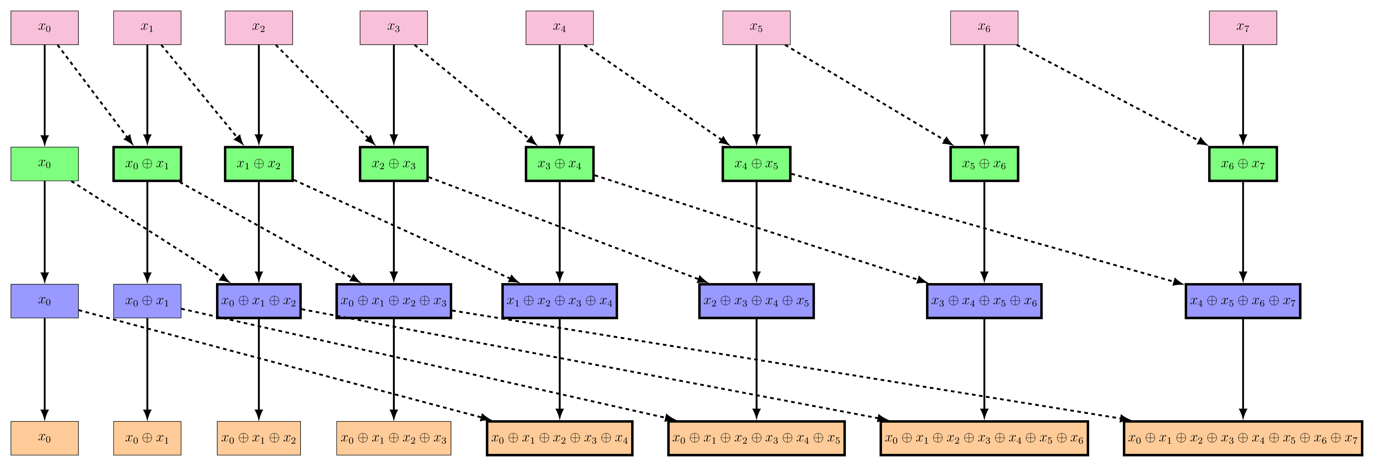Figure 3: The Hillis-Steele algorithm tree structure. Each level of the tree corresponds to a step in the computation of the scan operation. The nodes with a thicker border represent the new operations that are performed at each level. The top row is the input sequence $x$, and the bottom row is the output sequence $y$.

What makes this algorithm parallelizable is that at each level of the tree, we can compute the new values in parallel, because each operation at a given level only depends on the values from the previous level, and there are no dependencies between the operations at the same level.

If we implement this algorithm in C, we can use the OpenMP library to parallelize the operations at each level of the tree:

# | title: Hillis-Steele scan implementation
void hillis_steele(double *input, double *output, int n, double (*op)(double, double)) {
    // Allocate two buffers
    double *buffer1 = (double *)malloc(n * sizeof(double));
    double *buffer2 = (double *)malloc(n * sizeof(double));

    // Copy input to the first buffer
    memcpy(buffer1, input, n * sizeof(double));

    double *in = buffer1;
    double *out = buffer2;

    for (int d = 1; d < n; d *= 2) {
        #pragma omp parallel for
        for (int i = 0; i < n; i++) {
            if (i >= d)
                out[i] = op(in[i - d], in[i]);
            else
                out[i] = in[i];
        }
        // Swap buffers
        double *tmp = in;
        in = out;
        out = tmp;
    }

    // Copy the final result to output
    memcpy(output, in, n * sizeof(double));

    free(buffer1);
    free(buffer2);
}

We say that the Hillis-Steele algorithm is not work-efficient because it performs more operations than necessary. Indeed, at each level $d$ of the tree, we apply the operator $\oplus$ on $n-2^d$ elements, which means that we perform $n-2^d$ operations at each level. In total, we have a work complexity of $\bigO(n \log_2(n))$, which is worse than the naive implementation that has a work complexity of $\bigO(n)$. However, the parallel time complexity is $\bigO(\log_2(n))$, which is much better than the naive implementation that has a time complexity of $\bigO(n)$. Let’s see how this implementation performs in practice:

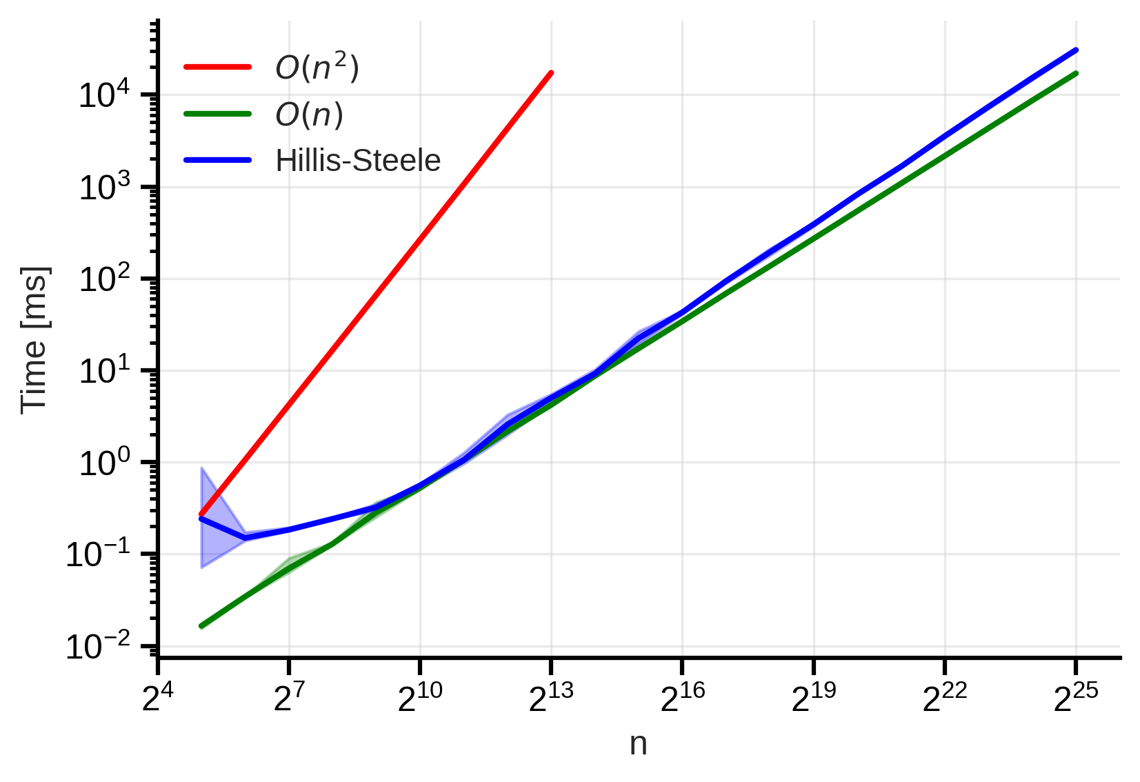Figure 4: Hillis-Steele scan time complexity. We observe strange results compared to the theory.

— Wait a minute ! This is absolutely not what we expected! The time complexity is not logarithmic ! It’s even worse than the naive implementation!

You’re right, this is not what we expected. We can try to understand what happened. First, it can be that our coding skills are not good enough to implement the algorithm correctly or that the overhead of the OpenMP library is too high. However, the main reason is probably that we live in a world where we have a limited number of processing units.

The bottleneck of the Hillis-Steele algorithm is that it requires a lot of processing units to be able to perform all operations in parallel. Indeed, to truly get the logarithmic time complexity, we need to have at least $n$ processing units available such that we can perform really “do in parallel”.

In practice, we often have a limited number of processing units available, let’s say $p$. In this case, the time complexity of the Hillis-Steele algorithm becomes $\bigO\left(\frac{n}{p} \log_2(n)\right)$. So because we don’t have enough processing units, the fact that the algorithm is not work-efficient does matter and rise the actual time complexity to be worse than the naive implementation.⁴

Fortunately, there is a better algorithm that is work-efficient and that can be parallelized: the Blelloch algorithm.

The Blelloch algorithm

The Blelloch algorithm is a more sophisticated algorithm that is both work-efficient and parallelizable. It can be described in two phases: the up-sweep phase and the down-sweep phase. The up-sweep phase is similar to the Hillis-Steele algorithm, but it is more efficient in terms of work complexity. The down-sweep phase is where we compute the final output sequence $y$ from the intermediate results computed during the up-sweep phase.

Up-sweep phase

The up-sweep phase is similar to the Hillis-Steele algorithm. At each level $d$ of the tree, we apply the $\oplus$ operator on pair of elements, and we store the result in the next level of the tree. The tree structure is as follows:

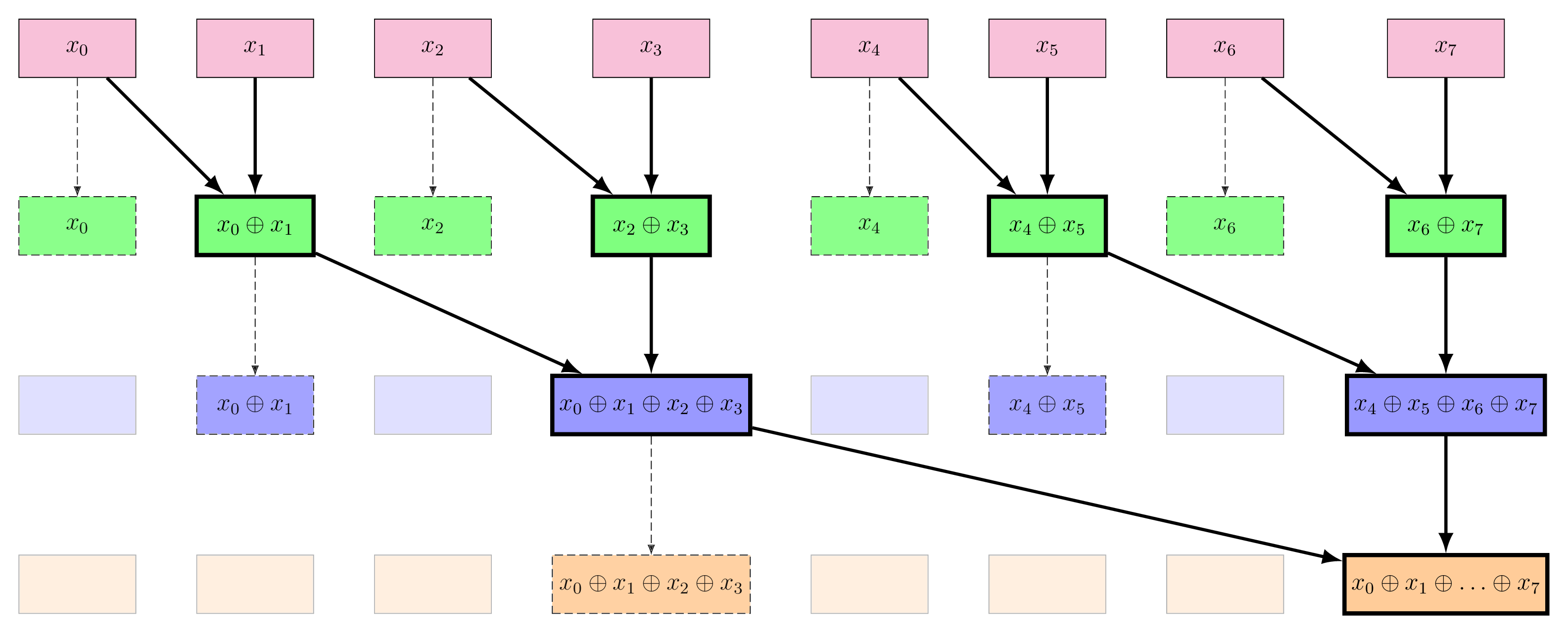Figure 5: The Blelloch algorithm up-sweep structure. Each level of the tree corresponds to a step in the computation of the scan operation. The nodes with a thicker border represent the new operations that are performed at each level. The top row is the input sequence $x$. Dashed structures should be ignored for the moment.

We can observe that at the end of the up-sweep phase, we have computed the last element of the output sequence $y$, which is the result of applying the operator $\oplus$ on all elements of the input sequence $x$. We can also observe that the up-sweep phase is work-efficient. Indeed at each level $d$ of the tree, we apply the operator $\oplus$ on $\dfrac{n}{2^{d+1}}$ pairs of elements, which means that we perform $\dfrac{n}{2^{d+1}}$ operations at each level. In total, we have a work complexity of $\bigO(n)$, which is the same as the naive implementation. The parallel time complexity is $\bigO(\log_2(n))$, which is the same as the Hillis-Steele algorithm.

However, in the scan operation, we want to compute all elements of the output sequence $y$, not just the last one. This is where the down-sweep phase comes into play.

Down-sweep phase

The down-sweep phase is where we compute the final output sequence $y$ from the intermediate results computed during the up-sweep phase. The down-sweep phase follows a pattern that can be harder to grasp at first. It involves understanding two things: (1) the pattern of the operations, and (2) what are the elements on which we apply the operations.

The down-sweep operator is as follows:

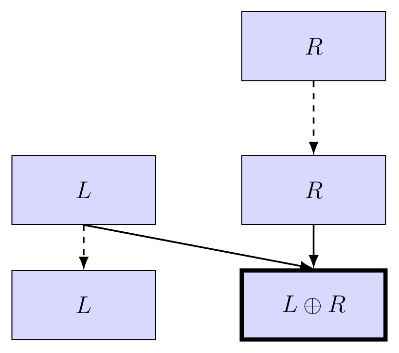Figure 6: The Blelloch algorithm down-sweep operator. The top row represents the two input elements $L$ and $R$. The bottom row represents the two output elements $R$ and $L \oplus R$. The operator takes two input elements and produces two output elements. The left output element is simply the left input element, while the right output element is the result of applying the operator $\oplus$ on the two input elements.

We are going to apply this operator at each level of the tree we built during the up-sweep phase. The dashed elements in the up-sweep tree structure represent the elements that we are going to use during the down-sweep phase. If at a given level, an element doesn’t fit within the operator, we simply copy it. The tree structure is as follows:

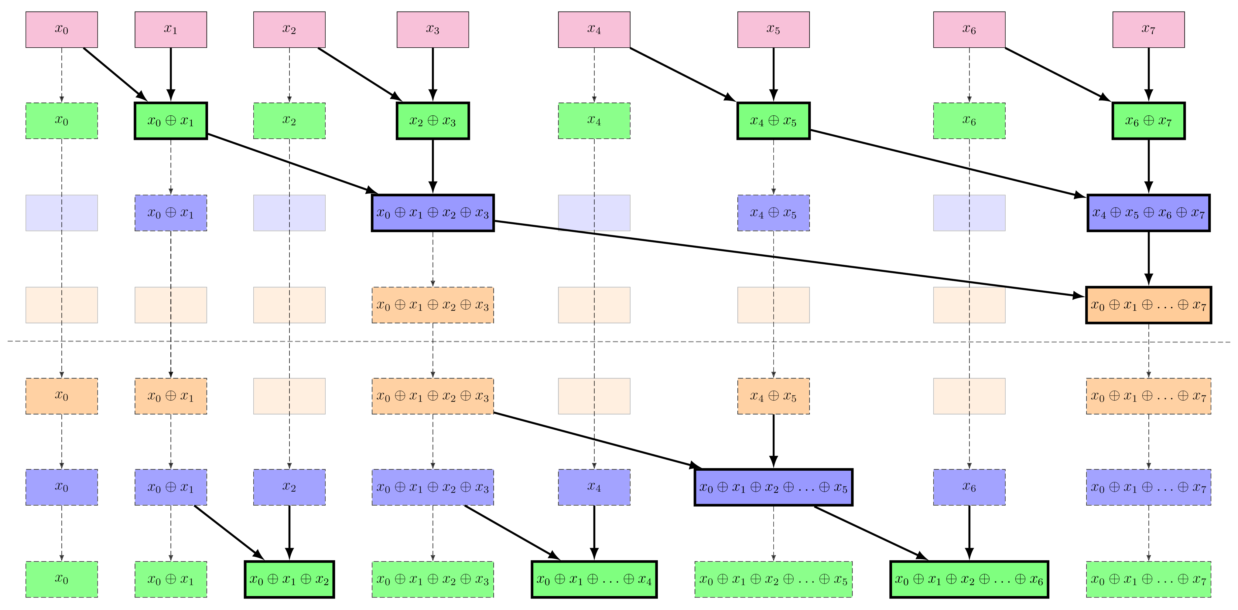Figure 7: The Blelloch algorithm down-sweep structure. Each level of the tree corresponds to a step in the computation of the scan operation. The nodes with a thicker border represent the new operations that are performed at each level. The top row is the input sequence $x$, and the bottom row is the output sequence $y$.

The tree structure presented here is a bit complex because we perform the inclusive scan. We also make the choice to not use an identity element for the operator $\oplus$. This means that we have to handle the first element of the output sequence $y$ differently. In this case, we simply copy the first element of the input sequence $x$ to the first element of the output sequence $y$.⁵ Note that the last element of the output sequence $y$ is not computed during the down-sweep phase and is just copied from the up-sweep phase.

We observe that the down-sweep phase is also work-efficient. The total work complexity is $\bigO(n)$, and the parallel time complexity is $\bigO(\log_2(n))$. The overall work complexity of the Blelloch algorithm is $\bigO(n)$, and the overall parallel time complexity is $\bigO(\log_2(n))$.

Here is a simple implementation of the Blelloch algorithm in C:

# | title: Blelloch scan implementation
void blelloch_scan_inclusive(double *input, double *output, int n, double (*op)(double, double)) {
    memcpy(output, input, n * sizeof(double));

    // Up-sweep (reduce) phase
    for (int d = 1; d < n; d *= 2) {
        #pragma omp parallel for
        for (int i = 0; i < n; i += 2 * d) {
            if (i + 2 * d - 1 < n) {
                output[i + 2 * d - 1] = op(output[i + d - 1], output[i + 2 * d - 1]);
            }
        }
    }

    // We do an inclusive scan, that's why this doesn't look like the usual Blelloch
    // Down-sweep phase
    for (int d = n / 2; d > 1; d /= 2) {
        #pragma omp parallel for
        for (int i = d; i < n; i += d) {
            output[i + d / 2 - 1] = op(output[i - 1], output[i + d / 2 - 1]);
        }
    }
}

We can see how this implementation performs in practice: 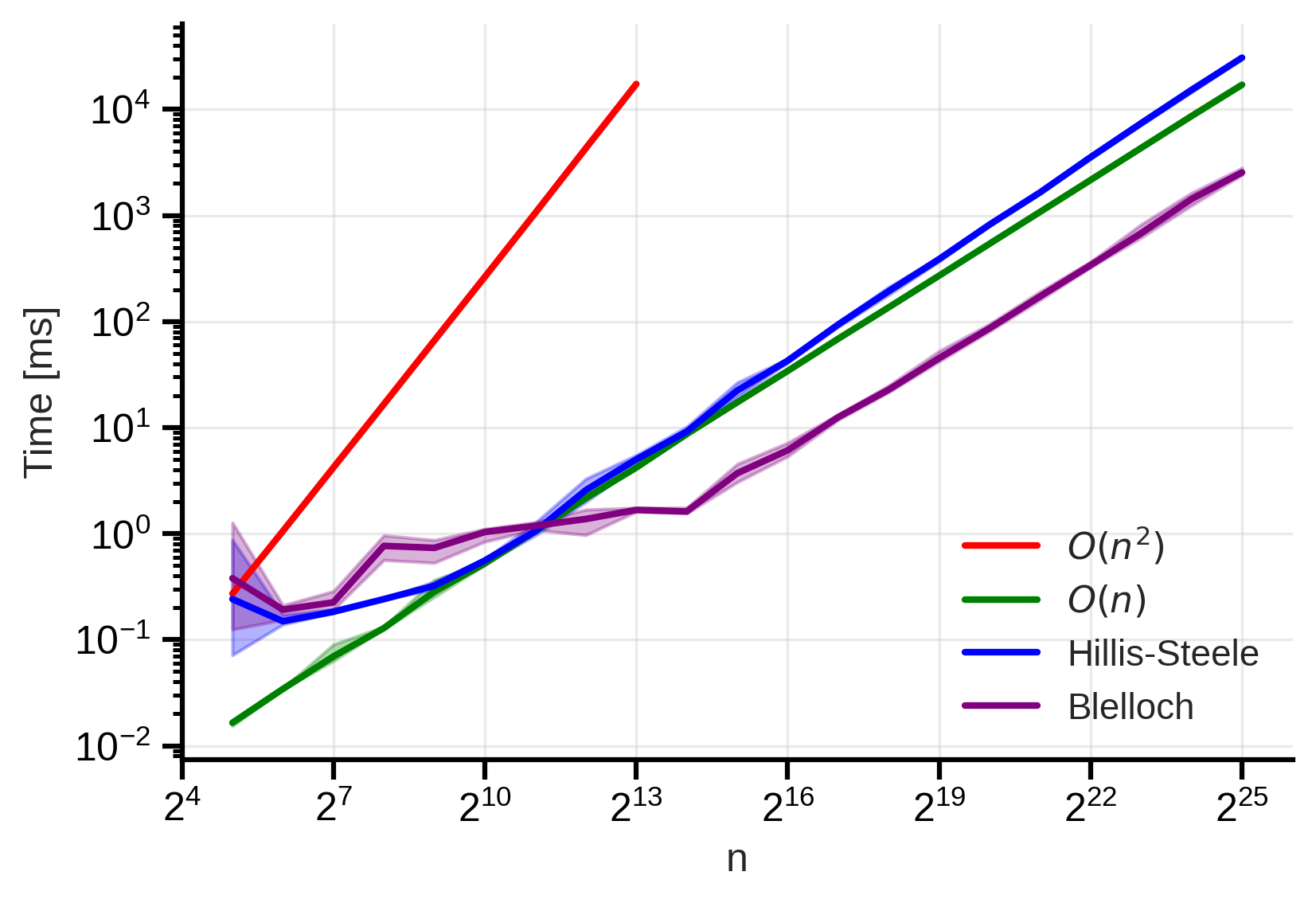Figure 8: Blelloch scan time complexity. We observe that it is better than the naive implementation and the Hillis-Steele algorithm. The shaded area shows the min-max variability across 5 different runs.

We can see that the Blelloch algorithm performs better than both the naive implementation and the Hillis-Steele algorithm. This is because it is both work-efficient and parallelizable. However, we can also observe that the time complexity is not logarithmic, which is probably due to the limited number of processing units available.

GPU implementations

Finally, it is worth mentioning that the scan operation is widely used in GPU programming. Indeed, what currently hinders the performance of the Hillis-Steele and Blelloch algorithms is the limited number of processing units available. On a GPU, we have a much larger number of processing units available, which allows us to fully exploit the parallelism of these algorithms. Here is a simple implementation of the Blelloch algorithm in CUDA for GPUs:

__device__ __forceinline__
double op_dev(double a, double b) {
    #pragma unroll 1
    for (int i = 0; i < ITER; i++) {
        a = a*a - 0.5*a + 0.1;
        b = b*b - 0.5*b + 0.1;
    }
    return a + b;
}

__global__ void upsweep_kernel(double* data, int n, int d) {
    int stride = 2 * d;
    long long tid = blockIdx.x * 1LL * blockDim.x + threadIdx.x;
    long long base = tid * 1LL * stride;

    if (base + stride - 1 < n) {
        double a = data[base + d - 1];
        double b = data[base + stride - 1];
        data[base + stride - 1] = op_dev(a, b);
    }
}

__global__ void downsweep_kernel(double* data, int n, int d) {
    int stride = d;
    long long tid = blockIdx.x * 1LL * blockDim.x + threadIdx.x;
    long long i = (tid + 1LL) * stride;

    if (i < n) {
        int left  = int(i - 1);
        int right = int(i + d/2 - 1);
        if (right < n) {
            double a = data[left];
            double b = data[right];
            data[right] = op_dev(a, b);
        }
    }
}

void blelloch_scan_inclusive_cuda(double *input, double *output, int n) {
    double *d_in, *d_out;
    cudaMalloc(&d_in,  n * sizeof(double));
    cudaMalloc(&d_out, n * sizeof(double));

    cudaMemcpy(d_in, input, n * sizeof(double), cudaMemcpyHostToDevice);
    cudaMemcpy(d_out, input, n * sizeof(double), cudaMemcpyHostToDevice);

    const int block = 256;

    for (int d = 1; d < n; d <<= 1) {
        int numSeg = (n + (2*d) - 1) / (2*d);
        int grid = (numSeg + block - 1) / block;
        upsweep_kernel<<<grid, block>>>(d_out, n, d);
    }

    for (int d = n >> 1; d > 1; d >>= 1) {
        int numI = (n + d - 1) / d;
        int grid = (numI + block - 1) / block;
        downsweep_kernel<<<grid, block>>>(d_out, n, d);
    }

    cudaMemcpy(output, d_out, n * sizeof(double), cudaMemcpyDeviceToHost);
    cudaFree(d_in);
    cudaFree(d_out);
}

The objective of this blog post is not to explain how to program in CUDA, so we will not go into the details of this implementation. Also, I’m not expert in CUDA, so maybe this is not the best implementation. However, we can see how this implementation performs in practice: 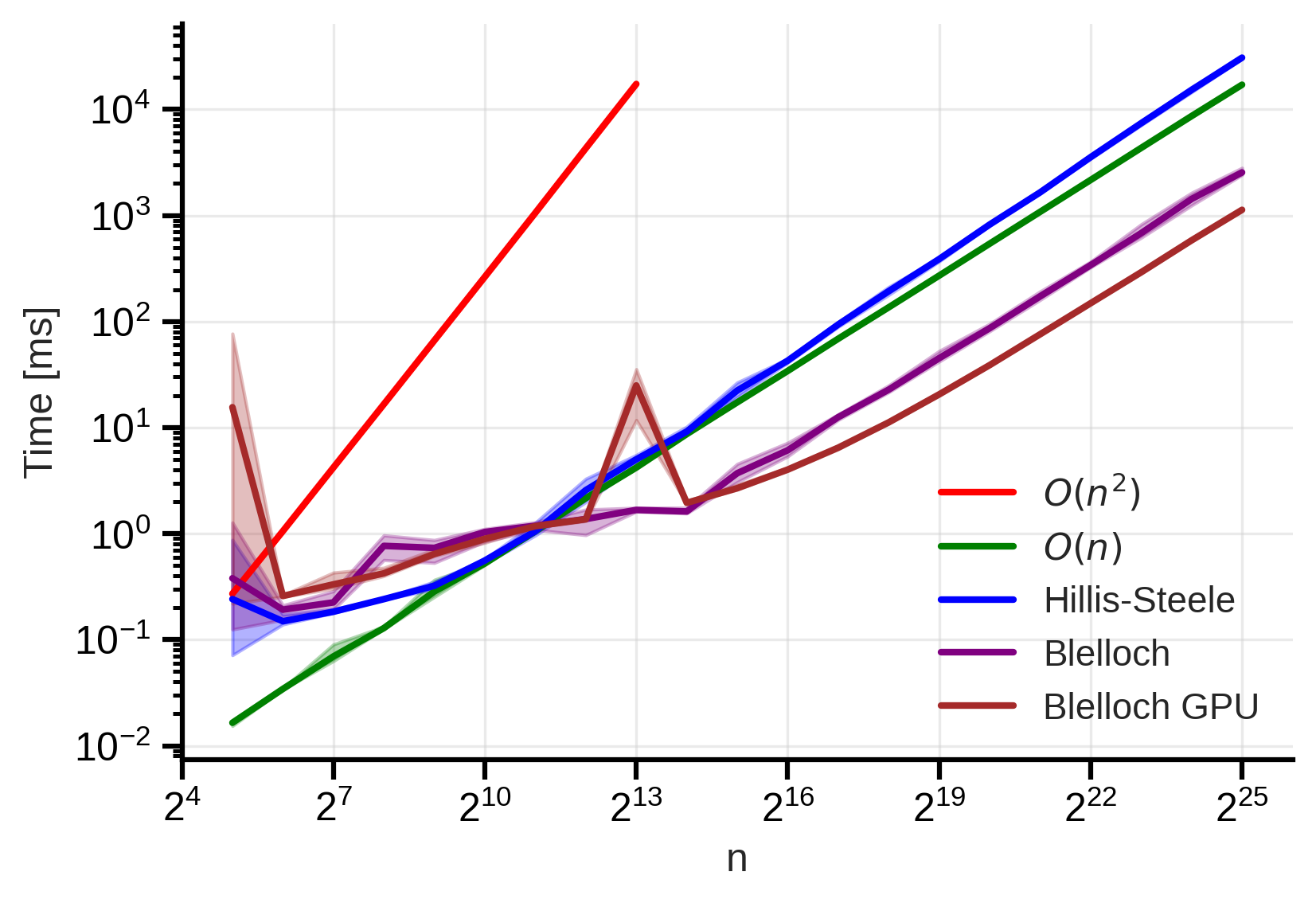Figure 9: Blelloch scan CUDA time complexity. We observe that we get the best performance with the GPU implementation. The shaded area shows the min-max variability across 5 different runs.

We can see that the GPU implementation of the Blelloch algorithm performs the best. This is because we have a much larger number of processing units available on a GPU, which allows us to fully exploit the parallelism of the algorithm for large input sizes.

Conclusion

In this blog post, we have explored the scan operation and how it can be parallelized. We have seen that the scan operation is not purely sequential and that it can be parallelized using the Hillis-Steele and Blelloch algorithms. We have also seen that the Blelloch algorithm is both work-efficient and parallelizable, which makes it a better choice for parallelizing the scan operation. Finally, we have seen that the scan operation is widely used in GPU programming, where we have a much larger number of processing units available to fully exploit the parallelism of the algorithm.

There are many more details that are not covered in this blog post, such as the exclusive scan, how to handle input sizes that are not powers of two, how to deal with memory accesses, block sizes, and many more. As usual when it comes to numerical methods and algorithms, the devil is in the details and a good practice is certainly not to implement these algorithms from scratch for something else than learning purposes, but rather to use well-tested libraries.

Some references for further reading:

1. M. Harris, Parallel Prefix Sum (Scan) with CUDA. NVIDIA Corporation, 2007. [Online]. Available: https://developer.download.nvidia.com/assets/cuda/files/reduction.pdf

2. G. E. Blelloch, “Prefix sums and their applications,” Technical Report CMU-CS-90-190, Carnegie Mellon University, 1990. [Online]. Available: https://www.cs.cmu.edu/~guyb/papers/Ble93.pdf

Appendix : why am I interested in the scan operation?

The reason I’m trying to understand the scan operation is because it appears in the context of parallelization of recurrent neural networks (RNNs). Since we need to be able to reformulate the RNN equations as an associative operation, this is not always possible, but when it is, we can use the scan operation to parallelize the computation of the RNN over time steps. Examples of such RNNs include state-space models (SSMs) and their variants. Some references:

1. Albert Gu, Karan Goel, and Christopher Ré, Efficiently Modeling Long Sequences with Structured State Spaces, 2022. arXiv:2111.00396

2. Albert Gu and Tri Dao, Mamba: Linear-Time Sequence Modeling with Selective State Spaces, 2024. arXiv:2312.00752

Appendix : benchmark code

The code used to benchmark the different implementations of the scan operation is available on GitHub. It includes the naive implementation, the Hillis-Steele algorithm, and the Blelloch algorithm for both CPU (using OpenMP) and GPU (using CUDA). The benchmark results are also available in the same folder.

footnotes

1. An associative operator is an operator that satisfies the property $(a \oplus b) \oplus c = a \oplus (b \oplus c)$ for all $a, b, c$. We do not emphasize more on this property in the following, but it is crucial for the scan operation to work correctly in parallel. Examples of associative operators include addition, multiplication, and logical operations like AND and OR. ↩︎

2. The scan operation is also known as the prefix sum in many contexts, especially in parallel computing literature. This is because the output sequence $y$ can be interpreted as a prefix sum of the input sequence $x$ when the operator $\oplus$ is addition. However, the scan operation is more general and can be applied with any associative operator. ↩︎

3. The scan operation comes in two flavors: exclusive and inclusive. The exclusive scan does not include the current element in the computation, while the inclusive scan does. In the example above, we have described the inclusive scan, where $y_i$ includes $x_i$ in its computation. In the rest of this post, we will focus on the inclusive scan, but the concepts can be easily adapted to the exclusive scan given an identity element for the operator $\oplus$. ↩︎

4. Here we are running the algorithm on CPUs so we have a “really small number” for $p$ ($p = 20$); On a GPU, we would have a much larger number of processing units available, and the Hillis-Steele algorithm would perform much better. However, the work complexity would still be worse than the naive implementation and for very long sequences, the Hillis-Steele algorithm would still be slower than the naive implementation. ↩︎

5. We decided to not use an identity element for the operator $\oplus$ because it is not always possible to define an identity element for a given operator. The only requirement for the operator $\oplus$ is to be associative. ↩︎